Fmri Spm 2nd Level Model Continuous Regressor

Statistical Parametric Mapping

Karl J Friston

Wellcome Dept. of Imaging Neuroscience

Contents

1. Introduction

2. Functional specialization and integration

3. Spatial realignment and normalisation

4. Statistical Parametric Mapping

5. Experimental design

6. Designing fMRI studies

7. Inferences about subjects and populations

8. Effective Connectivity

9. References

4. Statistical Parametric Mapping

Functional mapping studies are usually analyzed with some form of statistical parametric mapping. Statistical parametric mapping refers to the construction of spatially extended statistical processes to test hypotheses about regionally specific effects (Friston et al 1991). Statistical parametric maps (SPMs) are image processes with voxel values that are, under the null hypothesis, distributed according to a known probability density function, usually the Student's T or F distributions. These are known colloquially as T- or F-maps. The success of statistical parametric mapping is due largely to the simplicity of the idea. Namely, one analyses each and every voxel using any standard (univariate) statistical test. The resulting statistical parameters are assembled into an image - the SPM. SPMs are interpreted as spatially extended statistical processes by referring to the probabilistic behavior of Gaussian fields (Adler 1981, Worsley et al 1992, Friston et al 1994a, Worsley et al 1996). Gaussian random fields model both the univariate probabilistic characteristics of a SPM and any non-stationary spatial covariance structure. 'Unlikely' excursions of the SPM are interpreted as regionally specific effects, attributable to the sensorimotor or cognitive process that has been manipulated experimentally.

Over the years statistical parametric mapping has come to refer to the conjoint use of the general linear model (GLM) and Gaussian random field (GRF) theory to analyze and make classical inferences about spatially extended data through statistical parametric maps (SPMs). The GLM is used to estimate some parameters that could explain the data in exactly the same way as in conventional analysis of discrete data. GRF theory is used to resolve the multiple comparison problem that ensues when making inferences over a volume of the brain. GRF theory provides a method for correcting p values for the search volume of a SPM and plays the same role for continuous data (i.e. images) as the Bonferonni correction for the number of discontinuous or discrete statistical tests.

The approach was called SPM for three reasons; (i) To acknowledge Significance Probability Mapping, the use of interpolated pseudo-maps of p values used to summarize the analysis of multi-channel ERP studies. (ii) For consistency with the nomenclature of parametric maps of physiological or physical parameters (e.g. regional cerebral blood flow rCBF or volume rCBV parametric maps). (iii) In reference to the parametric statistics that comprise the maps. Despite its simplicity there are some fairly subtle motivations for the approach that deserve mention. Usually, given a response or dependent variable comprising many thousands of voxels one would use multivariate analyses as opposed to the mass-univariate approach that SPM represents. The problems with multivariate approaches are that; (i) they do not support inferences about regionally specific effects, (ii) they require more observations than the dimension of the response variable (i.e. number of voxels) and (iii), even in the context of dimension reduction, they are usually less sensitive to focal effects than mass-univariate approaches. A heuristic argument, for their relative lack of power, is that multivariate approaches estimate the model's error covariances using lots of parameters (e.g. the covariance between the errors at all pairs of voxels). In general, the more parameters (and hyper-parameters) an estimation procedure has to deal with, the more variable the estimate of any one parameter becomes. This renders inferences about any single estimate less efficient.

An alternative approach would be to consider different voxels as different levels of an experimental or treatment factor and use classical analysis of variance, not at each voxel (c.f. SPM), but by considering the data sequences from all voxels together, as replications over voxels. The problem here is that regional changes in error variance, and spatial correlations in the data, induce profound non-sphericity ¹ in the error terms. This non-sphericity would again require large numbers of [hyper]parameters to be estimated for each voxel using conventional techniques. In SPM the non-sphericity is parameterized in the most parsimonious way with just two [hyper]parameters for each voxel. These are the error variance and smoothness estimators (see Section IV.B and Figure 2). This minimal parameterization lends SPM a sensitivity that usually surpasses other approaches. SPM can do this because GRF theory implicitly imposes constraints on the non-sphericity implied by the continuous and [spatially] extended nature of the data. This is the only constraint on the behavior of the error terms implied by the use of GRF theory and is something that conventional multivariate and equivalent univariate approaches are unable to accommodate, to their cost.

Some analyses use statistical maps based on non-parametric tests that eschew distributional assumptions about the data. These approaches may, in some instances, be useful but are generally less powerful (i.e. less sensitive) than parametric approaches (see Aguirre et al 1998). Their original motivation in fMRI was based on the [specious] assumption that the residuals were not normally distributed. Next we consider parameter estimation in the context of the GLM. This is followed by an introduction to the role of GRF theory when making classical inferences about continuous data.

4.1 The general linear model

Statistical analysis of imaging data corresponds to (i) modeling the data to partition observed neurophysiological responses into components of interest, confounds and error and (ii) making inferences about the interesting effects in relation to the error variance. This inference can be regarded as a direct comparison of the variance due to an interesting experimental manipulation with the error variance (c.f. the F statistic and other likelihood ratios). Alternatively, one can view the statistic as an estimate of the response, or difference of interest, divided by an estimate of its standard deviation. This is a useful way to think about the T statistic.

A brief review of the literature may give the impression that there are numerous ways to analyze PET and fMRI time-series with a diversity of statistical and conceptual approaches. This is not the case. With very a few exceptions, every analysis is a variant of the general linear model. This includes; (i) simple T tests on scans assigned to one condition or another, (ii) correlation coefficients between observed responses and boxcar stimulus functions in fMRI, (iii) inferences made using multiple linear regression, (iv) evoked responses estimated using linear time invariant models and (v) selective averaging to estimate event-related responses in fMRI. Mathematically they are all identical. The use of the correlation coefficient deserves special mention because of its popularity in fMRI (Bandettini et al 1993). The significance of a correlation is identical to the significance of the equivalent T statistic testing for a regression of the data on the stimulus function. The correlation coefficient approach is useful but the inference is effectively based on a limiting case of multiple linear regression that obtains when there is only one regressor. In fMRI many regressors usually enter into a statistical model. Therefore, the T statistic provides a more versatile and generic way of assessing the significance of regional effects and is preferred over the correlation coefficient.

The general linear model is an equation that expresses the observed response variable Y in terms of a linear combination of explanatory variables X plus a well behaved error term (see Figure 3 and Friston et al 1995b). The general linear model is variously known as 'analysis of covariance' or 'multiple regression analysis' and subsumes simpler variants, like the 'T test' for a difference in means, to more elaborate linear convolution models such as finite impulse response (FIR) models. The matrix X that contains the explanatory variables (e.g. designed effects or confounds) is called the design matrix. Each column of the design matrix corresponds to some effect one has built into the experiment or that may confound the results. These are referred to as explanatory variables, covariates or regressors. The example in Figure 1 relates to a fMRI study of visual stimulation under four conditions. The effects on the response variable are modeled in terms of functions of the presence of these conditions (i.e. boxcars smoothed with a hemodynamic response function) and constitute the first four columns of the design matrix. There then follows a series of terms that are designed to remove or model low frequency variations in signal due to artifacts such as aliased biorhythms and other drift terms. The final column is whole brain activity. The relative contribution of each of these columns is assessed using standard least squares and inferences about these contributions are made using T or F statistics, depending upon whether one is looking at a particular linear combination (e.g. a subtraction), or all of them together. The operational equations are depicted schematically in Figure 3. In this scheme the general linear model has been extended (Worsley and Friston 1995) to incorporate intrinsic non-sphericity, or correlations among the error terms, and to allow for some specified temporal filtering of the data. This generalization brings with it the notion of effective degrees of freedom, which are less than the conventional degrees of freedom under i.i.d. assumptions (see footnote). They are smaller because the temporal correlations reduce the effective number of independent observations. The T and F statistics are constructed using Satterthwaite's approximation. This is the same approximation used in classical non-sphericity corrections such as the Geisser-Greenhouse correction. However, in the Worsley and Friston (1995) scheme, Satherthwaite's approximation is used to construct the statistics and appropriate degrees of freedom, not simply to provide a post hoc correction to the degrees of freedom.

The equations summarized in Figure 3 can be used to implement a vast range of statistical analyses. The issue is therefore not so much the mathematics but the formulation of a design matrix X appropriate to the study design and inferences that are sought. The design matrix can contain both covariates and indicator variables. Each column of X has an associated unknown parameter. Some of these parameters will be of interest (e.g. the effect of particular sensorimotor or cognitive condition or the regression coefficient of hemodynamic responses on reaction time). The remaining parameters will be of no interest and pertain to confounding effects (e.g. the effect of being a particular subject or the regression slope of voxel activity on global activity). Inferences about the parameter estimates are made using their estimated variance. This allows one to test the null hypothesis that all the estimates are zero using the F statistic to give an SPM{F} or that some particular linear combination (e.g. a subtraction) of the estimates is zero using a SPM{T}. The T statistic obtains by dividing a contrast or compound (specified by contrast weights) of the ensuing parameter estimates by the standard error of that compound. The latter is estimated using the variance of the residuals about the least-squares fit. An example of a contrast weight vector would be [-1 1 0 0..... ] to compare the difference in responses evoked by two conditions, modeled by the first two condition-specific regressors in the design matrix. Sometimes several contrasts of parameter estimates are jointly interesting. For example, when using polynomial (Büchel et al 1996) or basis function expansions of some experimental factor. In these instances, the SPM{F} is used and is specified with a matrix of contrast weights that can be thought of as a collection of 'T contrasts' that one wants to test together. A 'F-contrast' may look like,

which would test for the significance of the first or second parameter estimates. The fact that the first weight is -1 as opposed to 1 has no effect on the test because the F statistic is based on sums of squares.

. In most analysis the design matrix contains indicator variables or parametric variables encoding the experimental manipulations. These are formally identical to classical analysis of [co]variance (i.e. AnCova) models. An important instance of the GLM, from the perspective of fMRI, is the linear time invariant (LTI) model. Mathematically this is no different from any other GLM. However, it explicitly treats the data-sequence as an ordered time-series and enables a signal processing perspective that can be very useful.

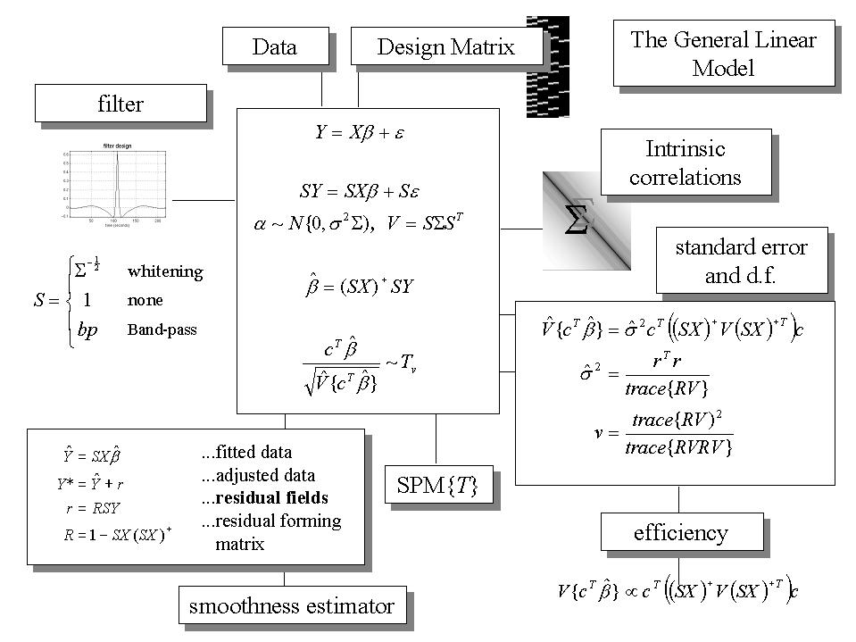
Figure 3. The general linear model. The general linear model is an equation expressing the response variable Y in terms of a linear combination of explanatory variables in a design matrix X and an error term with assumed or known autocorrelation ?. In fMRI the data can be filtered with a convolution matrix S, leading to a generalized linear model that includes [intrinsic] serial correlations and applied [extrinsic] filtering. Different choices of S correspond to different [de]convolution schema as indicated on the upper left. The parameter estimates obtain in a least squares sense using the pseudoinverse (denoted by +) of the filtered design matrix. Generally an effect of interest is specified by a vector of contrast weights c that give a weighted sum or compound of parameter estimates referred to as a contrast. The T statistic is simply this contrast divided by its the estimated standard error (i.e. square root of its estimated variance). The ensuing T statistic is distributed with v degrees of freedom. The equations for estimating the variance of the contrast and the degrees of freedom associated with the error variance are provided in the right-hand panel. Efficiency is simply the inverse of the variance of the contrast. These expressions are useful when assessing the relative efficiency of an experimental design. The parameter estimates can either be examined directly or used to compute the fitted responses (see lower left panel). Adjusted data refers to data from which estimated confounds have been removed. The residuals r obtain from applying the residual-forming matrix R to the data. These residual fields are used to estimate the smoothness of the component fields of the SPM used in Gaussian random field theory (see Figure 6).

4.1.1 Linear Time Invariant (LTI) systems and temporal basis functions

In Friston et al (1994b) the form of the hemodynamic impulse response function (HRF) was estimated using a least squares de-convolution and a time invariant model, where evoked neuronal responses are convolved with the HRF to give the measured hemodynamic response (see also Boynton et al 1996). This simple linear framework is the cornerstone for making statistical inferences about activations in fMRI with the GLM. An impulse response function is the response to a single impulse, measured at a series times after the input. It characterizes the input-output behavior of the system (i.e.. voxel) and places important constraints on the sorts of inputs that will excite a response. The HRFs, estimated in Friston et al (1994b) resembled a Poisson or Gamma function, peaking at about 5 seconds. Our understanding of the biophysical and physiological mechanisms that underpin the HRF has grown considerably in the past few years (e.g. Buxton and Frank 1997). Figure 4 shows some simulations based on the hemodynamic model described in Friston et al (2000a). Here, neuronal activity induces some auto-regulated signal that causes transient increases in rCBF. The resulting flow increases dilate the venous balloon increasing its volume (v) and diluting venous blood to decrease deoxyhemoglobin content (q). The BOLD signal is roughly proportional to the concentration of deoxyhemoglobin (q/v) and follows the rCBF response with about a seconds delay.

Knowing the forms that the HRF can take is important for several reasons, not least because it allows for better statistical models of the data. The HRF may vary from voxel to voxel and this has to be accommodated in the GLM. To allow for different HRFs in different brain regions the notion of temporal basis functions, to model evoked responses in fMRI, was introduced (Friston et al 1995c) and applied to event-related responses in Josephs et al (1997) (see also Lange and Zeger 1997). The basic idea behind temporal basis functions is that the hemodynamic response induced by any given trial type can be expressed as the linear combination of several [basis] functions of peristimulus time. The convolution model for fMRI responses takes a stimulus function encoding the supposed neuronal responses and convolves it with a HRF to give a regressor that enters into the design matrix. When using basis functions the stimulus function is convolved with all the basis functions to give a series of regressors. The associated parameter estimates are the coefficients or weights that determine the mixture of basis functions that best models the HRF for the trial type and voxel in question. We find the most useful basis set to be a canonical HRF and its derivatives with respect to the key parameters that determine its form (e.g. latency and dispersion). The nice thing about this approach is that it can partition differences among evoked responses into differences in magnitude, latency or dispersion, that can be tested for using specific contrasts and the SPM{T} (see Friston et al 1998b for details).

Temporal basis functions are important because they enable a graceful transition between conventional multi-linear regression models with one stimulus function per condition and FIR models with a parameter for each time point following the onset of a condition or trial type. Figure 5 illustrates this graphically (see Figure legend). In summary, temporal basis functions offer useful constraints on the form of the estimated response that retain (i) the flexibility of FIR models and (ii) the efficiency of single regressor models. The advantage of using several temporal basis functions (as opposed to an assumed form for the HRF) is that one can model voxel-specific forms for hemodynamic responses and formal differences (e.g. onset latencies) among responses to different sorts of events. The advantages of using basis functions over FIR models are that (i) the parameters are estimated more efficiently and (ii) stimuli can be presented at any point in the inter-stimulus interval. The latter is important because time-locking stimulus presentation and data acquisition gives a biased sampling over peristimulus time and can lead to differential sensitivities, in multi-slice acquisition, over the brain.

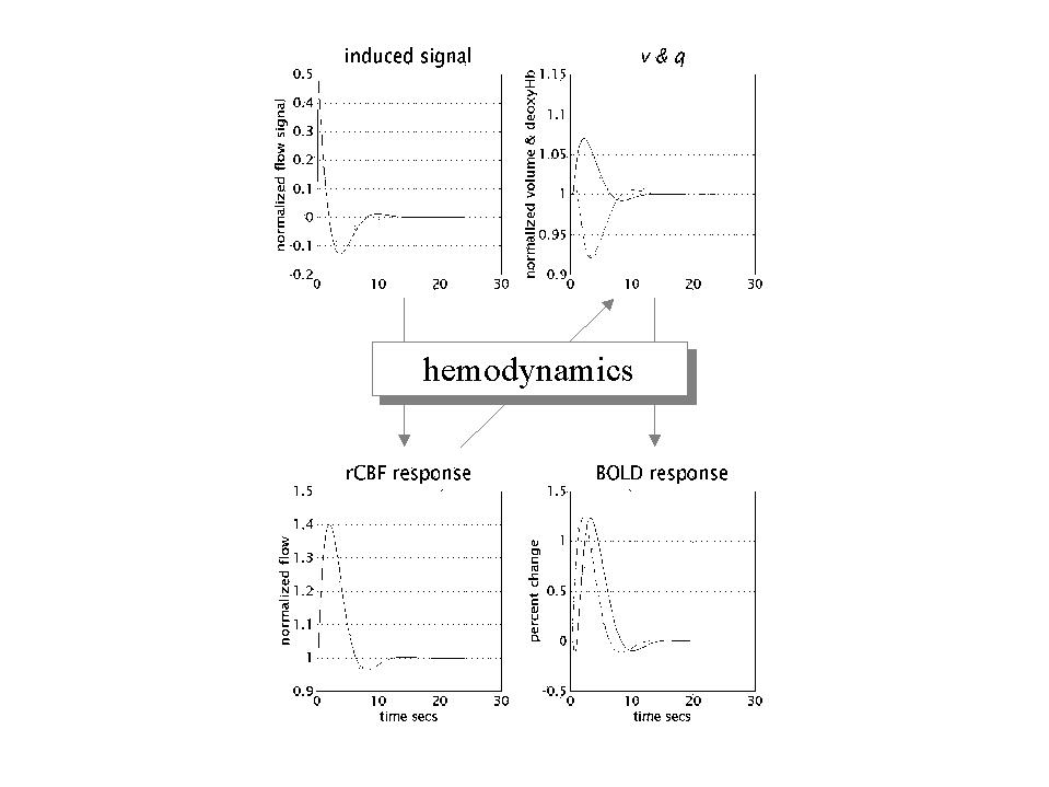
Figure 4. Hemodynamics elicited by an impulse of neuronal activity as predicted by a dynamical biophysical model (see Friston et al 2000a for details). A burst of neuronal activity causes an increase in flow inducing signal that decays with first order kinetic and is down regulated by local flow. This signal increases rCBF with dilates the venous capillaries increasing its volume (v). Concurrently, venous blood is expelled from the venous pool decreasing deoxyhemoglobin content (q). The resulting fall in deoxyhemoglobin concentration leads to a transient increases in BOLD (blood oxygenation level dependent) signal and a subsequent undershoot.

4.2 Statistical inference and the theory of Gaussian fields

Inferences using SPMs can be of two sorts depending on whether one knows where to look in advance. With an anatomically constrained hypothesis, about effects in a particular brain region, the uncorrected p value associated with the height or extent of that region in the SPM can be used to test the hypothesis. With an anatomically open hypothesis (i.e. a null hypothesis that there is no effect anywhere in a specified volume of the brain) a correction for multiple dependent comparisons is necessary. The theory of Gaussian random fields provides a way of correcting the p-value that takes into account the fact that neighboring voxels are not independent by virtue of continuity in the original data. Provided the data are sufficiently smooth the GRF correction is less severe (i.e. is more sensitive) than a Bonferroni correction for the number of voxels. As noted above GRF theory deals with the multiple comparisons problem in the context of continuous, spatially extended statistical fields, in a way that is analogous to the Bonferroni procedure for families of discrete statistical tests. There are many ways to appreciate the difference between GRF and Bonferroni corrections. Perhaps the most intuitive is to consider the fundamental difference between a SPM and a collection of discrete T values. When declaring a connected volume or region of the SPM to be significant, we refer collectively to all the voxels that comprise that volume. The false positive rate is expressed in terms of connected [excursion] sets of voxels above some threshold, under the null hypothesis of no activation. This is not the expected number of false positive voxels. One false positive volume may contain hundreds of voxels, if the SPM is very smooth. A Bonferroni correction would control the expected number of false positive voxels, whereas GRF theory controls the expected number of false positive regions. Because a false positive region can contain many voxels the corrected threshold under a GRF correction is much lower, rendering it much more sensitive. In fact the number of voxels in a region is somewhat irrelevant because it is a function of smoothness. The GRF correction discounts voxel size by expressing the search volume in terms of smoothness or resolution elements (Resels). See Figure 6. This intuitive perspective is expressed formally in terms of differential topology using the Euler characteristic (Worsley et al 1992). At high thresholds the Euler characteristic corresponds to the number of regions exceeding the threshold.

There are only two assumptions underlying the use of the GRF correction: (i) The error fields (but not necessarily the data) are a reasonable lattice approximation to an underlying random field with a multivariate Gaussian distribution. (ii) These fields are continuous, with a twice-differentiable autocorrelation function. A common misconception is that the autocorrelation function has to be Gaussian. It does not. The only way in which these assumptions can be violated is if; (i) the data are not smoothed (with or without sub-sampling of the data to preserve resolution), violating the reasonable lattice assumption or (ii) the statistical model is mis-specified so that the errors are not normally distributed. Early formulations of the GRF correction were based on the assumption that the spatial correlation structure was wide-sense stationary. This assumption can now be relaxed due to a revision of the way in which the smoothness estimator enters the correction procedure (Kiebel et al 1999). In other words, the corrections retain their validity, even if the smoothness varies from voxel to voxel.

4.2.1 Anatomically closed hypotheses

When making inferences about regional effects (e.g. activations) in SPMs, one often has some idea about where the activation should be. In this instance a correction for the entire search volume is inappropriate. However, a problem remains in the sense that one would like to consider activations that are 'near' the predicted location, even if they are not exactly coincident. There are two approaches one can adopt; (i) pre-specify a small search volume and make the appropriate GRF correction (Worsley et al 1996) or (ii) used the uncorrected p value based on spatial extent of the nearest cluster (Friston 1997). This probability is based on getting the observed number of voxels, or more, in a given cluster (conditional on that cluster existing). Both these procedures are based on distributional approximations from GRF theory.

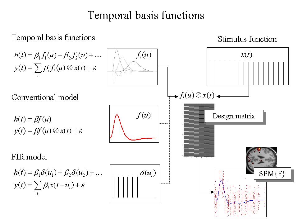
Figure 5. Temporal basis functions offer useful constraints on the form of the estimated response that retain (i) the flexibility of FIR models and (ii) the efficiency of single regressor models. The specification of these constrained FIR models involves setting up stimulus functions x(t) that model expected neuronal changes [e.g. boxcars of epoch-related responses or spikes (delta functions) at the onset of specific events or trials]. These stimulus functions are then convolved with a set of basis functions of peri-stimulus time u, that model the HRF, in some linear combination. The ensuing regressors are assembled into the design matrix. The basis functions can be as simple as a single canonical HRF (middle), through to a series of delayed delta functions (bottom). The latter case corresponds to a FIR model and the coefficients constitute estimates of the impulse response function at a finite number of discrete sampling times, for the event or epoch in question. Selective averaging in event-related fMRI (Dale and Buckner 1997) is mathematically equivalent to this limiting case.

4.2.2 Anatomically open hypotheses and levels of inference

To make inferences about regionally specific effects the SPM is thresholded, using some height and spatial extent thresholds that are specified by the user. Corrected p-values can then be derived that pertain to; (i) the number of activated regions (i.e. number of clusters above the height and volume threshold) - set level inferences, (ii) the number of activated voxels (i.e. volume) comprising a particular region - cluster level inferences and (iii) the p-value for each voxel within that cluster - voxel level inferences. These p-values are corrected for the multiple dependent comparisons and are based on the probability of obtaining c, or more, clusters with k, or more, voxels, above a threshold u in an SPM of known or estimated smoothness. This probability has a reasonably simple form (see Figure 6 for details).

Set-level refers to the inference that the number of clusters comprising an observed activation profile is highly unlikely to have occurred by chance and is a statement about the activation profile, as characterized by its constituent regions. Cluster-level inferences are a special case of set-level inferences, that obtain when the number of clusters c = 1. Similarly voxel-level inferences are special cases of cluster-level inferences that result when the cluster can be small (i.e. k = 0). Using a theoretical power analysis (Friston et al 1996b) of distributed activations, one observes that set-level inferences are generally more powerful than cluster-level inferences and that cluster-level inferences are generally more powerful than voxel-level inferences. The price paid for this increased sensitivity is reduced localizing power. Voxel-level tests permit individual voxels to be identified as significant, whereas cluster and set-level inferences only allow clusters or sets of clusters to be declared significant. It should be remembered that these conclusions, about the relative power of different inference levels, are based on distributed activations. Focal activation may well be detected with greater sensitivity using voxel-level tests based on peak height. Typically, people use voxel-level inferences and a spatial extent threshold of zero. This reflects the fact that characterizations of functional anatomy are generally more useful when specified with a high degree of anatomical precision.

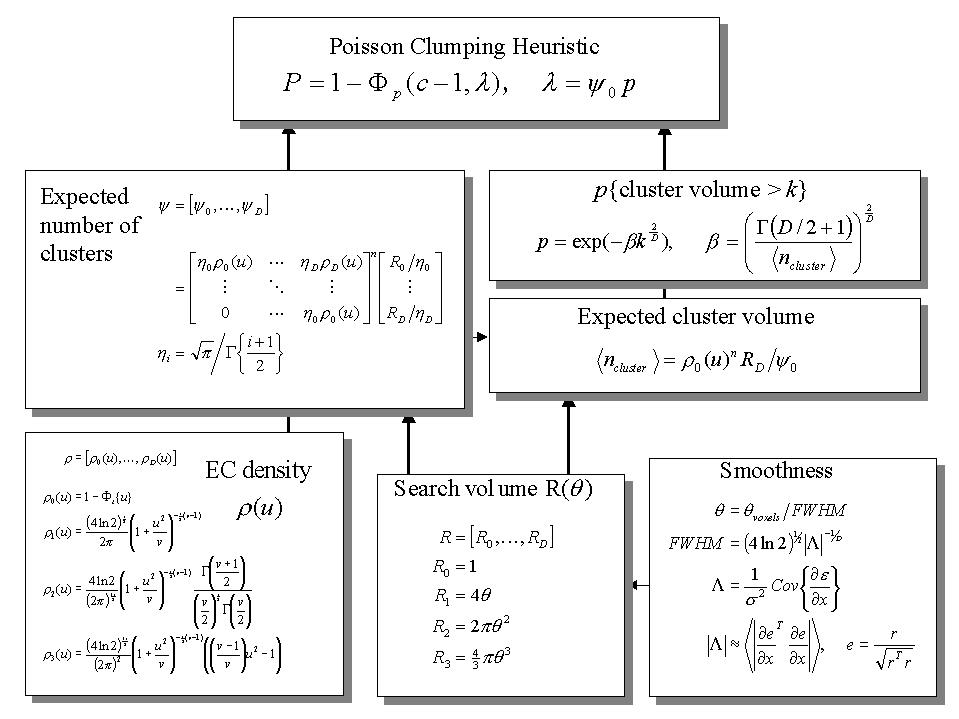
Figure 6. Schematic illustrating the use of Gaussian random field theory in making inferences about activations in SPMs. If one knew where to look exactly, then inference can be based on the value of the statistic at a specified location in the SPM, without correction. However, if one did not have an anatomical constraint a priori, then a correction for multiple dependent comparisons has to be made. These corrections are usually made using distributional approximations from GRF theory. This schematic deals with a general case of n SPM{T}s whose voxels all survive a common threshold u (i.e. a conjunction of n component SPMs). The central probability, upon which all voxel, cluster or set-level inferences are made is the probability P of getting c or more clusters with k or more resels (resolution elements) above this threshold. By assuming that clusters behave like a multidimensional Poisson point process (i.e. the Poisson clumping heuristic) P is simply determined. The distribution of c is Poisson with an expectation that corresponds to the product of the expected number of clusters, of any size, and the probability that any cluster will be bigger than k resels. The latter probability is shown using a form for a single Z-variate field constrained by the expected number of resels per cluster (<.> denotes expectation or average). The expected number of resels per cluster is simply the expected number of resels in total divided by the expected number of clusters. The expected number of clusters is estimated with the Euler characteristic (EC) (effectively the number of blobs minus the number of holes). This estimate is in turn a function of the EC density for the statistic in question (with degrees of freedom v) and the resel counts. The EC density is the expected EC per unit of D-dimensional volume of the SPM where the D dimensional volume of the search space is given by the corresponding element in the vector of resel counts. Resel counts can be thought of as a volume metric that has been normalized by the smoothness of the SPMs component fields expressed in terms of the full width at half maximum (FWHM). This is estimated from the determinant of the variance-covariance matrix of the first spatial derivatives of e, the normalized residual fields r (from Figure 3). In this example equations for a sphere of radius ? are given. ? denotes the cumulative density function for the sub-scripted statistic in question.

1 Sphericity refers to the assumption of identically and independently distributed error terms (i.i.d.). Under i.i.d. the probability density function of the errors, from all observations, has spherical iso-contours, hence sphericity. Deviations from either of the i.i.d. criteria constitute non-sphericity. If the error terms are not identically distributed then different observations have different error variances. Correlations among error terms reflect dependencies among the error terms (e.g. serial correlation in fMRI time series) and constitute the second component of non-sphericity.

campbelloffam1958.blogspot.com

Source: https://www.fil.ion.ucl.ac.uk/spm/course/notes02/overview/Stats.htm

Share this post